Sección 3.3 Plano Euclidiano
¶En esta seccion estudiaremos los planos métricos, que cumple en quinto axioma de Euclides. Dado ejemplo de la realizacion de estos planos Euclidianos
Subsección 3.3.1 Plano Euclidiano
¶El plano Euclidiano es un plano métrico en el cual se cumple el quinto postulado de Euclides, es decir, es un plano \(\Pi= (\mathcal{P}, \mathcal{L} \mathcal{I},\perp) \) que cumple con
Los axiomas afines
Los axiomas de ortogonalidad
Los axiomas de colinealidad
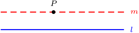
Axioma Euclides Si \(P\not\mathcal{I} l \) entonces \(\exists ! m \in \mathcal{L}\) tal que \(P \mathcal{I} m \ \wedge \ m \parallel l\)
Introducción:
A través de este axioma se derivan muchas propiedades de la geometría clásica, como las siguientes:
-
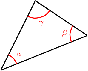
La suma de los ángulos interiores de un triángulo suman \(180^\circ\)
\begin{equation*}
\alpha+\beta+\gamma=180^\circ
\end{equation*}
-
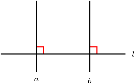
Si \(a\perp l \wedge b\perp l\text{,}\) \(a\neq b\) entonces \(a\parallel b\)
-
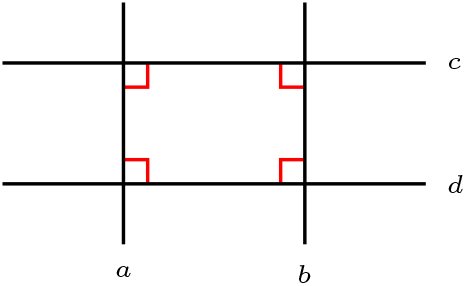
Si \(a\perp c \wedge a\perp d \text{,}\) \(b\perp c\) entonces \(b\perp d\)
-
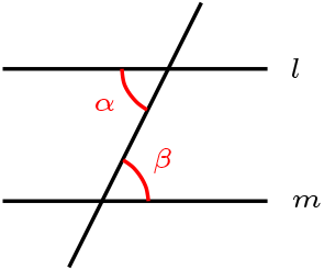
ángulos alternos internos
\begin{equation*}
l \parallel m \Rightarrow \alpha = \beta
\end{equation*}
-
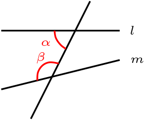
Si \(l \nparallel m \text{ entonces } \alpha + \beta \neq 180^\circ\)
Subsección 3.3.2 Modelos de Plano Euclidiano
¶Sean \(V\) un plano vectorial sobre \(\mathbb{K}\) tal que \(2\neq0\) y \(f:V \times V \rightarrow \mathbb{K}\text{,}\) una forma bilineal, simétrica sin vectores isótropos, es decir,
-
Bilineal:
Se dice que \(f\) es lineal en la primera componente.
- \((\forall\overrightarrow{v_1},\overrightarrow{v_2},\overrightarrow{v_3}
\in V)( f(\overrightarrow{v_1}+\overrightarrow{v_2},\overrightarrow{v_3})=
f(\overrightarrow{v_1},\overrightarrow{v_3})+f(\overrightarrow{v_2},\overrightarrow{v_3}))\text{.}\)
- \((\forall \alpha \in \mathbb{K})( \forall \overrightarrow{v},\overrightarrow{w}\in V)
( f(\alpha \overrightarrow{v},\overrightarrow{w})=\alpha f(\overrightarrow{v},\overrightarrow{w}))\)
Note que la linealidad en la segunda componente, se logra con la siguiente propiedad
-
Simétrica:
Se dice que \(f\) es simétrica si y sólo si
\begin{equation*}
(\forall \overrightarrow{v},\overrightarrow{w}\in V)( f(\overrightarrow{v},\overrightarrow{w})=f(\overrightarrow{w},\overrightarrow{v})).
\end{equation*}
-
Sin vectores isótropos:
Se dice que \(f\) no tiene vectores isótropos si y sólo si
\begin{equation*}
(\forall \overrightarrow{v} \in V ) (f(\overrightarrow{v},\overrightarrow{v})=0 \Rightarrow \overrightarrow{v}=0).
\end{equation*}
Plano Métrico Euclidiano
Sean \(V\) un plano vectorial y \(f:V \times V \rightarrow \mathbb{K}\text{,}\) una forma bilineal, simétrica sin vectores isótropos.
Definimos el plano \((V,f)\text{,}\) de modo que el conjunto de puntos es \(\mathcal{P}= V \text{,}\) el conjunto de recta \(\mathcal{L}\) es el conjunto de rectas afines, la incidencia \(\mathcal{I}\) es la pertenecía y la ortogonalidad entre rectas esta dada por
\begin{equation*}
\left\langle v_1 \right\rangle + w_1 \perp \left\langle v_2 \right\rangle+w_2 \text{ si y sólo si } f(v_1,v_2)=0.
\end{equation*}
Proposición 3.3.1
Sea \(V\) un \(\mathbb{K}\)-espacio vectorial y \(f\) un forma bilineal simétrica sin vectores isótropos, entonces \((V,f)\) es un Plano Métrico Euclidiano
Demostración
De ejercicios los axiomas afines y de ortogonalidad, recordar para ello las nociones de geometría analítica, el de colineación lo veremos mas adelante.
Ejemplo 3.3.2
Sea \((\mathbb{R}^2,f)\) plano Euclidiano, con \(f\) el producto interno usual, es decir,
\begin{equation*}
\begin{array}{cccc}
f: \amp \mathbb{R}^2 \times \mathbb{R}^2 \amp \rightarrow \amp \mathbb{R}\\
\amp ((x_1,x_2),(y_1,y_2)) \amp \rightsquigarrow \amp x_1 x_2 +y_1 y_2
\end{array}
\end{equation*}
Dada las rectas \(l_1:y=x+2 \text{ y } l_2:y=-x-3\text{.}\)
Determine si \(l_1 \perp l_2\text{.}\)
Para el caso real, con el producto usual sabemos que
\begin{equation*}
l_1 \perp l_2 \Leftrightarrow m_1 \cdot m_2 =-1
\end{equation*}
lo cual es verdadero.
De otro modo, o en general con un producto arbitrario, tenemos
\begin{equation*}
l_1= \left \langle (1,1) \right \rangle +(0,2) ;\ \ l_2= \left \langle (1,-1) \right \rangle + (0,-3)
\end{equation*}
Evaluando el vector director
\begin{equation*}
f((1,1),(1,-1))=1 \cdot 1 + 1\cdot -1 = 0
\end{equation*}
Por lo tanto
\begin{equation*}
l_1 \perp l_2.
\end{equation*}
Ejemplo 3.3.4
Sea \(\mathbb{K}=\mathbb{Z}_5\) y \(V=\mathbb{Z}_5 \times \mathbb{Z}_5\) y la forma bilineal simétrica sin vectores isótropos
\begin{equation*}
f((x_1,x_2),(y_1,y_2))=x_1 x_2 + 3 y_1 y_2=x_1 x_2 -2 y_1 y_2.
\end{equation*}
Determine si \(l_1=\left\langle (1,\ 1) \right\rangle+(2,3)\) y \(l_2=\{ (x,y) \in V \ | \ x-2y=1 \}\) son ortogonales.
Sea \((x,y) \in l_2\) entonces
\begin{equation*}
(x,y)=(1+2y,y)=y(2,1)+(1,0)
\end{equation*}
luego \(l_2: \left\langle (2,\ 1) \right\rangle +(1,0)\text{,}\) entonces
\begin{equation*}
f((1,1),(2,1))=2+3=5=0 \ \in \mathbb{Z}_5
\end{equation*}
por lo tanto \(l_1 \perp l_2\text{.}\)
Subsección 3.3.3 Colineaciones del Plano Euclidiano
¶Sea \((V,f)\) un plano Euclidiano y \(g: V \rightarrow V\) una transformación lineal invertible, hemos visto que preservan incidencia, ahora veremos la ortogonalidad.
Se dice que \(g\) es una isometría si y sólo si
\begin{equation*}
(\forall v,w \in V)( f(g(v), g(w))=f(u,v) )
\end{equation*}
Note que la ortogonalidad esta definida a partir de la forma bilineal, luego una isometría son colineaciones. Claramente la identidad es una isometría
Se define el grupo ortogonal de \((V,f)\) igual a
\begin{equation*}
O(f) = \{ g : V \rightarrow V \ | \ g \text{ es una isometría } \}
\end{equation*}
Caso particular Sea \((\mathbb{R}^2, f)\) con la formal usual tenemos que
\begin{equation*}
f(x,y) = x_1y_1+x_2y_2 = [x_1 \ x_2]
\left(\begin{array}{cc} 1 \amp 0 \\ 0 \amp 1 \end{array}\right)
\left[\begin{array}{c} y_1 \\ y_2 \end{array} \right]
\end{equation*}
Una forma de explicitar las isometrías es matrimonialmente, para ello consideramos una base la base canónica \(C\) y calculemos
\begin{equation*}
\begin{array}{rcl}
f(g(v), g(w))\amp=\amp f(u,v) \\
{[g(v)]}^t_C [f]_C [g(w)]_C\amp=\amp {[u]^t_C}[f]_C[v]_C \\
([g]_C[v]_C)^t [f]_C[g]_C[w]v\amp=\amp {[u]^t_C}[f]_C[v]_C \\
{[v]^t_C} {[g]^t_C} [f]_C[g]_C[w]_C\amp=\amp {[u]^t_C}[f]_C[v]_C
\end{array}
\end{equation*}
Es una igualdad para todo los vectores, por lo tanto
\begin{equation*}
{[g]^t_C} [f]_C[g]_C=[f]_C
\end{equation*}
Si \(g\) es una isometría tal que \(A= [g]_C \text{,}\) reemplazando obtenemos que
\begin{equation*}
A^tA= I_2
\end{equation*}
Grupo de las matrices ortogonales de \(2 \times 2\)
\begin{equation*}
O(f) = \{A\in GL_2(\mathbb{R}) \ | \ A^tA= I \}.
\end{equation*}
Para explicitar directamente este grupo. Sea
\begin{equation*}
A= \left(\begin{array}{cc} a \amp b \\ c \amp d \end{array}\right)
\end{equation*}
La ecuación matricial \(A^tA=I\text{,}\) nos entrega el sistema de ecuaciones
\begin{equation*}
\begin{array}{ccc|}
a^2+c^2 \amp = \amp 1 \\
b^2+d^2 \amp = \amp 1 \\
ab+cd \amp = \amp 0 \\ \hline
\end{array}
\end{equation*}
Ya que los puntos pertenecen al circunferencia unitaria, podemos parametrizar
\begin{equation*}
a= cos(\alpha); \ c = sen(\alpha),\ b= cos(\beta); \ d = sen(\beta)
\end{equation*}
luego se cumple las dos primeras ecuaciones y la tercera
\begin{equation*}
0= cos(\alpha)cos(\beta)+sen(\alpha)sen(\beta)= cos(\beta-\alpha)
\end{equation*}
de lo cual obtenemos
\begin{equation*}
\beta -\alpha = \frac{\pi}{2}+ 2k\pi \text{ o bien }\beta -\alpha = \frac{3\pi}{2}+ 2k\pi
\end{equation*}
Veamos la primera posibilidad y reemplacemos
\begin{equation*}
a= cos(\alpha); \ c = sen(\alpha),\ b= cos(\frac{\pi}{2} + \alpha); \ d = sen(\frac{\pi}{2} + \alpha)
\end{equation*}
Utilizando identidades, finalmente obtenemos que
\begin{equation*}
A= \left(\begin{array}{cc} cos(\alpha) \amp-sen(\alpha) \\sen(\alpha) \amp cos(\alpha) \end{array}\right)
\end{equation*}
matriz de tienen determinante 1 y corresponde a rotaciones en un ángulo \(\alpha.\)
En la otra posibilidad se obtiene
\begin{equation*}
A= \left(\begin{array}{cc} cos(\alpha) \amp sen(\alpha) \\ sen(\alpha) \amp -cos(\alpha) \end{array}\right)
\end{equation*}
matriz de tiene determinante -1.
Luego tenemos el grupo ortogonal esta formado por
\begin{equation*}
O(f) =\left \{\left(\begin{array}{cc} cos(\alpha) \amp-sen(\alpha) \\sen(\alpha) \amp cos(\alpha) \end{array}\right),
\left(\begin{array}{cc} cos(\alpha) \amp sen(\alpha) \\ sen(\alpha) \amp -cos(\alpha) \end{array}\right) \ | \ \alpha \in [0,2\pi] \right\}.
\end{equation*}
Note que las matrices de determinante -1, dejan fijos todos los punto de la recta
\begin{equation*}
\lt (cos(\alpha)+1, sen(\alpha))\gt ,
\end{equation*}
por lo anterior es una simetría entorno a la recta, ya que al cuadrado es la identidad.
Al multiplicar dos de esta simetrías obtenemos
\begin{equation*}
\left(\begin{array}{cc}
cos(\alpha) \amp sen(\alpha) \\ sen(\alpha) \amp -cos(\alpha) \end{array}\right)
\left(\begin{array}{cc}
cos(\beta) \amp sen(\beta) \\ sen(\beta) \amp -cos(\beta) \end{array}\right)
=\left(\begin{array}{cc}
cos(\alpha-\beta) \amp -sen(\alpha-\beta) \\ sen(\alpha-\beta) \amp cos(\alpha-\beta) \end{array}\right)
\end{equation*}
una rotación, que son las otras matrices del grupo ortogonal, los otros axiomas se obtiene en forma similar.
Luego tenemos el grupo ortogonal de las rotaciones esta formado por:
\begin{equation*}
O^+(f) =\left \{\left(\begin{array}{cc} cos(\alpha) \amp-sen(\alpha) \\ sen(\alpha) \amp cos(\alpha) \end{array}\right) \ | \ \alpha \in [0,2\pi] \right\}.
\end{equation*}
Subsección 3.3.4 Simetrías
¶Notemos que la recta fija anterior no tiene una expresión comoda, por ello determinaremos en forma explícita la simetría respecto a la recta \(l \in \mathcal{L}\) .
Primer Caso: Cuando la Recta es Vectorial.
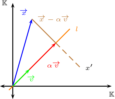
Sean \(l=\left \langle \overrightarrow{v} \right \rangle\text{,}\) \(\overrightarrow{x}\in V\) y \(R_l\) simetrías de eje \(l\text{.}\)
Determinemos primero \(\alpha \in \mathbb{K}\) tal que \(x-\alpha \overrightarrow{v}\text{,}\) sea ortogonal a \(l\)
\begin{equation*}
f(\overrightarrow{x}-\alpha \overrightarrow{v},\overrightarrow{v})=0
\end{equation*}
\begin{equation*}
\begin{array}{rcl}
f(\overrightarrow{x}-\alpha \overrightarrow{v},\overrightarrow{v}) \amp = \amp 0 \\
f(\overrightarrow{x},\overrightarrow{v})-\alpha f(\overrightarrow{v},\overrightarrow{v}) \amp = \amp 0 \\
\alpha f(\overrightarrow{v},\overrightarrow{v})\amp = \amp f(\overrightarrow{x},\overrightarrow{v})
\end{array}
\end{equation*}
Luego tenemos
\begin{equation*}
\alpha = \frac{f(\overrightarrow{x},\overrightarrow{v})}{f(\overrightarrow{v},\overrightarrow{v})}
\end{equation*}
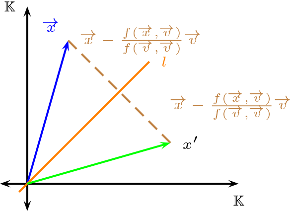
\begin{equation*}
\begin{array}{rcl}
x'\amp =\amp \overrightarrow{x}-2(\overrightarrow{x}-\frac{f(\overrightarrow{x},\overrightarrow{v})}{f(\overrightarrow{v},\overrightarrow{v})} \cdot \overrightarrow{v})\\
x' \amp =\amp - \overrightarrow{x}+2\frac{f(\overrightarrow{x},\overrightarrow{v})}{f(\overrightarrow{v},\overrightarrow{v})} \cdot \overrightarrow{v}
\end{array}
\end{equation*}
De este modo tenemos que la simetría esta dada por:
\begin{equation*}
R_{l}(\overrightarrow{x})=-\overrightarrow{x}+2\frac{f(\overrightarrow{x},\overrightarrow{v})}{f(\overrightarrow{v},\overrightarrow{v})} \cdot \overrightarrow{v}
\end{equation*}
Segundo Caso: La recta no es vectorial.
Sean \(l=\left \langle \overrightarrow{v}\right \rangle + \overrightarrow{w}, \overrightarrow{x}\in V\) y \(R_l\) simetrías de eje \(l\text{.}\)
Si \(\overrightarrow{P} \mathcal{I} l\) entonces, existe \(\alpha_1 \in \mathbb{K}\) tal que \(\overrightarrow{P}= \alpha_1 \overrightarrow{v}+\overrightarrow{w}\)
\begin{equation*}
\begin{array}{rcl}
R_l(\alpha_1 \overrightarrow{v}+\overrightarrow{w}) \amp = \amp\alpha_1 \overrightarrow{v}+\overrightarrow{w} \\
(R_l \circ T_{\overrightarrow{w}})(\alpha_{1}\overrightarrow{v})\amp = \amp T_{\overrightarrow{w}} (\alpha_1\overrightarrow{v})\\
(T_{\overrightarrow{w}}^{-1} \circ R_l \circ T_{\overrightarrow{w}})(\alpha_{1}\overrightarrow{v})\amp = \amp \alpha_{1}\overrightarrow{v}
\end{array}
\end{equation*}
luego, \(T_{\overrightarrow{w}}^{-1} \circ R_l \circ T_{\overrightarrow{w}}\) tiene orden 2 y fija a todos los puntos de la forma \(\alpha_{1}\overrightarrow{v}\text{,}\) entonces:
\begin{equation*}
T_{\overrightarrow{w}}^{-1} \circ R_l \circ T_{\overrightarrow{w}}=Id \text{ }\vee \text{ } T_{\overrightarrow{w}}^{-1} \circ R_l \circ T_{\overrightarrow{w}}=R_{\left\langle \overrightarrow{v} \right\rangle}
\end{equation*}
Si \(T_{\overrightarrow{w}}^{-1} \circ R_l \circ T_{\overrightarrow{w}}=Id\text{,}\) despejando se tiene que \(R_l = Id\) lo cual es una contradicción, luego tenemos
\begin{equation*}
T_{\overrightarrow{w}}^{-1} \circ R_l \circ T_{\overrightarrow{w}}= R_{\left\langle \overrightarrow{v}\right\rangle}
\end{equation*}
del cual se establece que:
\begin{equation*}
R_l= T_{\overrightarrow{w}}\circ R_{\left \langle \overrightarrow{v}\right \rangle} \circ T_{\overrightarrow{w}}^{-1}
\end{equation*}
De este modo tenemos que la simetría esta dada por:
\begin{equation*}
R_{l}(\overrightarrow{x})=
-(\overrightarrow{x}-\overrightarrow{w})+2
\frac{f(\overrightarrow{x}-\overrightarrow{w},\overrightarrow{v})}{
f(\overrightarrow{v},\overrightarrow{v})} \cdot \overrightarrow{v}+\overrightarrow{w}
\end{equation*}
Proposición 3.3.5
Sea \((V,f)\) plano métrico euclidiano y la recta \(l = \lt \overrightarrow{v} \gt +\overrightarrow{w} \) entonces
\begin{equation*}
\begin{array}{crcc}
R_l:\amp V \amp\rightarrow \amp V \\
\amp \overrightarrow{x} \amp \rightsquigarrow \amp
2\overrightarrow{w} -\overrightarrow{x}+2 \frac{f(\overrightarrow{x}-\overrightarrow{w},\overrightarrow{v})}{ f(\overrightarrow{v},\overrightarrow{v}) } \cdot \overrightarrow{v}
\end{array}
\end{equation*}
Ejemplo 3.3.6
Sea \(\left ( \mathbb{R}^2, f\right )\) plano Euclidiano con el producto usual
\begin{equation*}
f((x_1,x_2),(y_1,y_2))=x_1 x_2 +y_1 y_2
\end{equation*}
Dada \(l:y=2x\text{,}\) Calcule \(R_l(x,y)\text{.}\)
Ya que \(l:y=2x\text{,}\) obtenemos \(l=\left\langle (1,2)\right\rangle\)
\begin{equation*}
\begin{array}{rcl}
R_l(x,y) \amp = \amp -(x,y)+2\frac{f((x,y),(1,2))}{f((1,2),(1,2))}\cdot (1,2)\\
R_l(x,y) \amp = \amp (-x,-y)+2 (\frac{x+2y}{5})\cdot (1,2) \\
R_l(x,y) \amp = \amp (-x,-y)+(\frac{2x+4y}{5},\frac{4x+8y}{5}) \\
R_l(x,y) \amp = \amp (\frac{-3x+4y}{5},\frac{4x+3y}{5})
\end{array}
\end{equation*}
En la base canónica \(C\text{,}\) se tiene que
\begin{equation*}
A=[R_l]_C= \left(\begin{array}{cc} -3/5 \amp 4/5 \\ 4/5 \amp3/5 \end{array}\right), \quad det(A)=-1.
\end{equation*}
Y la funcion esta definida por
\begin{equation*}
\begin{array}{crcc}
R_l:\amp \mathbb{R}^2 \amp\rightarrow \amp \mathbb{R}^2 \\
\amp (x,y) \amp \rightsquigarrow \amp
\frac{1}{5}(-3x+4y,4x+3y)
\end{array}
\end{equation*}
Ejemplo 3.3.7
Sea \((\mathbb{Z}_{7}^{2},f)\) plano euclidiano y la forma bilineal simétrica sin vectores isótropos.
\begin{equation*}
f((x_1,x_2),(y_1,y_2))=x_1 x_2 - \overline{5}y_1 y_2.
\end{equation*}
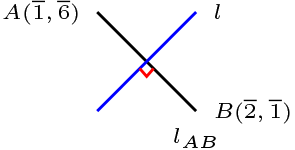
Sea \(l\) la recta tal que \(R_{l}(\overline{2},\overline{1})=(\overline{1},\overline{6})\text{.}\)
Determine \(R_{l}(x,y)\)
Para determinar la recta
\begin{equation*}
l=\left \langle \overrightarrow{v} \right \rangle + \overrightarrow{w}
\end{equation*}
veamos los siguiente:
\begin{equation*}
\begin{array}{rcl}
l_{AB} \amp = \amp \left \langle A-B \right \rangle + B \\
l_{AB} \amp = \amp \left \langle (\overline{1},\overline{6})-(\overline{2},\overline{1})\right \rangle + (\overline{2},\overline{1}) \\
l_{AB} \amp = \amp \left \langle (-\overline{1},\overline{5})\right \rangle + (\overline{2},\overline{1})
\end{array}
\end{equation*}
Pero \(l_{AB} \perp l\text{,}\) luego sean \((x_1,x_2)\in \left \langle \overrightarrow{v} \right \rangle \)
\begin{equation*}
\begin{array}{rcl}
f((x_1,x_2),(-\overline{1},\overline{5})) \amp = \amp 0 \\
-x_1-\overline{25}x_2 \amp = \amp 0 \\
x_1 \amp = \amp \overline{3}x_2
\end{array}
\end{equation*}
Entonces \((x_1,x_2)=(3x_2,x_2)=x_2(3,1)\text{,}\) por lo tanto \(l=\left \langle (\overline{3},\overline{1})\right \rangle + (c,d)\) Además \(w = (-a+2,5a+1)\text{,}\) reemplazando tenemos
\begin{equation*}
\begin{array}{rcl}
R_{l}(\overline{2},\overline{1})
\amp = \amp 2w- (\overline{2},\overline{1}) + \overline{2}\cdot
\frac{f((\overline{2},\overline{1})-w,(\overline{3},\overline{1}))}
{f((\overline{3},\overline{1}),(\overline{3},\overline{1}))}\cdot (\overline{3},\overline{1})\\
\amp = \amp (\overline{-2a+2},\overline{10a+1}) + \overline{4}\cdot f(-\overrightarrow{v},(\overline{3},\overline{1})) (\overline{3},\overline{1}) \\
\amp = \amp (\overline{-2a+2},\overline{10a+1}) + \overline{0}\cdot (\overline{3},\overline{1}) \\
\amp = \amp (\overline{-2a+2},\overline{10a+1})
\end{array}
\end{equation*}
note que el punto se obtiene de \(2w- (\overline{2},\overline{1})=(\overline{1},\overline{6})\) es decir el punto medio
\begin{equation*}
\begin{array}{ccc}
P_{m} \amp = \amp (\frac{\overline{2}+\overline{1}}{2}, \frac{\overline{1}+\overline{6}}{2}) \\
P_{m} \amp = \amp (3\cdot 3,3 \cdot 7) \\
P_{m} \amp = \amp (5,0)
\end{array}
\end{equation*}
Luego \(l=\left \langle (\overline{3},\overline{1})\right \rangle + (\overline{5},\overline{0})\text{.}\)
Finalmente podemos encontrar la reflexion dada por
\begin{equation*}
R_{l}(x,y)=2\overrightarrow{w} -\overrightarrow{x}+2 \frac{f(\overrightarrow{x}-\overrightarrow{w},\overrightarrow{v})}{ f(\overrightarrow{v},\overrightarrow{v}) } \cdot \overrightarrow{v}
\end{equation*}
\begin{equation*}
\begin{array}{rcl}
R_{l}(x,y)
\amp = \amp (\overline{10}-x,-y)+\overline{2}\cdot \frac{f((x-\overline{5},y),(\overline{3},\overline{1}))}{
f((\overline{3},\overline{1}),(\overline{3},\overline{1}))}\cdot (\overline{3},\overline{1})\\
\amp = \amp (\overline{10}-x,-y)+ \frac{(\overline{3}x-\overline{1}-\overline{5}y)}{\overline{2}}\cdot (\overline{3},\overline{1}) \\
\amp = \amp (\overline{10}-x,-y)+ \overline{4}\cdot(\overline{3}x-\overline{1}-\overline{5}y)\cdot (\overline{3},\overline{1}) \\
\amp = \amp (\overline{10}-x,-y)+(x+\overline{3}y+\overline{2},\overline{5}x+y+\overline{3}) \\
\amp = \amp \left ( \overline{3}y+\overline{7}+\overline{5},\overline{5}x+\overline{3}+\overline{0} \right ) \\
R_{l}(x,y) \amp = \amp \left ( \overline{3}y + \overline{5},\overline{5}x + \overline{3}\right )
\end{array}
\end{equation*}
Subsección 3.3.5 Traslaciones en el Plano Euclidiano
¶En el plano euclidiano real \((V,f)\text{,}\)
Sean \(b:\lt \overrightarrow{v} \gt + \overrightarrow{u} \) y \(d:\lt \overrightarrow{v} \gt + \overrightarrow{w} \) rectas afines.
Luego tenemos
\begin{equation*}
\begin{array}{ccl}
(R_b\circ R_d)(\overrightarrow{x}) \amp = \amp R_b( 2\overrightarrow{w}-\overrightarrow{x}+2 \frac{f(\overrightarrow{x}-\overrightarrow{w},\overrightarrow{v})}{ f(\overrightarrow{v},\overrightarrow{v}) } \cdot \overrightarrow{v}) \\
\amp = \amp \overrightarrow{x}+ 2\overrightarrow{u}-2\overrightarrow{w}+2\frac{f(\overrightarrow{w}-\overrightarrow{u},\overrightarrow{v})}{ f(\overrightarrow{v},\overrightarrow{v}) } \cdot \overrightarrow{v} \\
\amp = \amp t_{2\overrightarrow{u}-2\overrightarrow{w}+2\frac{f(\overrightarrow{w}-\overrightarrow{u},\overrightarrow{v})}{ f(\overrightarrow{v},\overrightarrow{v}) } \cdot \overrightarrow{v}} (\overrightarrow{x})
\end{array}
\end{equation*}
Notemos que
\begin{equation*}
f(2\overrightarrow{u}-2\overrightarrow{w}+2\frac{f(\overrightarrow{w}-\overrightarrow{u},\overrightarrow{v})}{ f(\overrightarrow{v},\overrightarrow{v}) } \cdot \overrightarrow{v}, \overrightarrow{v})=
2f(\overrightarrow{u}-\overrightarrow{w}, \overrightarrow{v})+
2\frac{f(\overrightarrow{w}-\overrightarrow{u},\overrightarrow{v})}{ f(\overrightarrow{v},\overrightarrow{v})}f( \overrightarrow{v}, \overrightarrow{v})=0
\end{equation*}
Por ellos es un traslación, en dirección de la recta ortogonal a \(b:\lt \overrightarrow{v} \gt \text{.}\)
Subsección 3.3.6 Rotaciones en el Plano Euclidiano
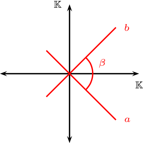
¶En el plano euclidiano real \((V,f)\text{,}\) sea \(\sigma\) una rotación de centro \(P\text{.}\)
Luego existen \(a ,b \in \mathcal{L}\) tal que \(a \cap b = \{P\}\) y \(\sigma = R_{a} \circ R_{b}\text{.}\)
Si \(P=\overrightarrow{0}\) y \(\alpha\) es el ángulo de rotación, si \(\beta\) es el ángulo entre \(a\) y \(b\) entonces
\begin{equation*}
\alpha = 2 \cdot \beta
\end{equation*}
\begin{equation*}
\sigma(x,y)= \begin{pmatrix}
\cos \alpha \amp - \sin \alpha \\
\sin \alpha \amp \cos \alpha
\end{pmatrix} \begin{pmatrix}
x \\
y
\end{pmatrix}
\end{equation*}
Formula para rotaciones de centro \((0,0)\) y ángulo \(\alpha\)
\begin{equation*}
\sigma(x,y)=( x\cos \alpha - y\sin \alpha, x\sin \alpha +y\cos \alpha )
\end{equation*}
Si \(P \neq \overrightarrow{0}\text{,}\) entonces las rotaciones de centro \(P\) y ángulo \(\alpha\) vienen dadas por la formula:
\begin{equation*}
\sigma(x,y)=\left ( T_{\overrightarrow{P}} \circ
\begin{pmatrix}
\cos \alpha \amp - \sin \alpha \\
\sin \alpha \amp \cos \alpha
\end{pmatrix} \circ T_{\overrightarrow{P}}^{-1} \right )(x,y)
\end{equation*}
Ejemplo 3.3.8
Sea \(\left ( \mathbb{R}^2, f\right )\) plano Euclidiano con el producto usual
\begin{equation*}
f((x_1,x_2),(y_1,y_2))=x_1 x_2 +y_1 y_2
\end{equation*}
Dadas las rectas \(l_1:y=5x\) y \(l_2: y=2x\text{.}\)
Determinar explícitamente la rotación \(R_{l_1}\circ R_{l_2}(x,y)\) y el ángulo de rotación .
Ya que \(l_1:x=5y\text{,}\) y \(l_2: y=2x\) obtenemos
\begin{equation*}
\begin{array}{rcl}
\sigma (x,y) \amp = \amp R_{l_1}\circ R_{l_2}(x,y) \\ \\
\amp=\amp R_{l_1}( -(x,y)+2\frac{f((x,y),(1,2))}{f((1,2),(1,2))}\cdot (1,2)\\ \\
\amp=\amp R_{l_1}(\frac{-3x+4y}{5},\frac{4x+3y}{5}) \\ \\
\amp=\amp -(\frac{-3x+4y}{5},\frac{4x+3y}{5})+\frac{1}{13} \frac{-11x+23y}{5}(5,1) \\ \\
\amp=\amp -(\frac{-3x+4y}{5},\frac{4x+3y}{5})+\frac{1}{13} \frac{-11x+23y}{5}(5,1) \\ \\
\amp=\amp (\frac{-16x+63y}{65},\frac{-63x-16y}{65})
\end{array}
\end{equation*}
Expresando en coordenadas de la base canónica, se tiene que
\begin{equation*}
[\sigma (x,y)]_C = \frac{1}{65}\begin{pmatrix}
-16 \amp 63 \\ -63 \amp -16 \end{pmatrix} \begin{pmatrix}
x \\ y \end{pmatrix}
\end{equation*}
De lo cual tenemos que
\begin{equation*}
\arctan (\frac{63}{16}) \approx 75,75^\circ.
\end{equation*}
Ya que \(\sigma(1,0)=(\frac{-16}{65},\frac{-63}{65})\) y \(\sigma(0,1)=(\frac{63}{65},\frac{-16}{65})\text{,}\) el ángulo es
\begin{equation*}
\alpha \approx -75,75^\circ.
\end{equation*}
Subsubsección Ejercicios
Sean \((V,f)\) plano euclidiano, \(a, b\in \mathcal{L}\) tal que \(a\cap b\not=\phi\text{.}\)
Determine la rotación, de centro \(P\) y
\begin{equation*}
\sigma= R_a\circ R_b
\end{equation*}
Subsubsección Ejercicios
Sean \((V,f)\) plano euclidiano, \(a, b\in \mathcal{L}\) tal que \(a\cap b\not=\phi\) y \(a\perp b\text{.}\)
Determine la simetría puntual, de centro \(P\)
\begin{equation*}
\sigma= R_a\circ R_b
\end{equation*}